Pose estimation is calculated by using computer vision to detect the position and orientation of an object. This usually means detecting key point locations that describe the object. For example, in the example of face pose estimation (a.k.a facial landmark detection), we detect landmarks on a human face. A related example is head pose estimation where we use the facial landmarks to obtain the 3D orientation of a human head with respect to the camera.
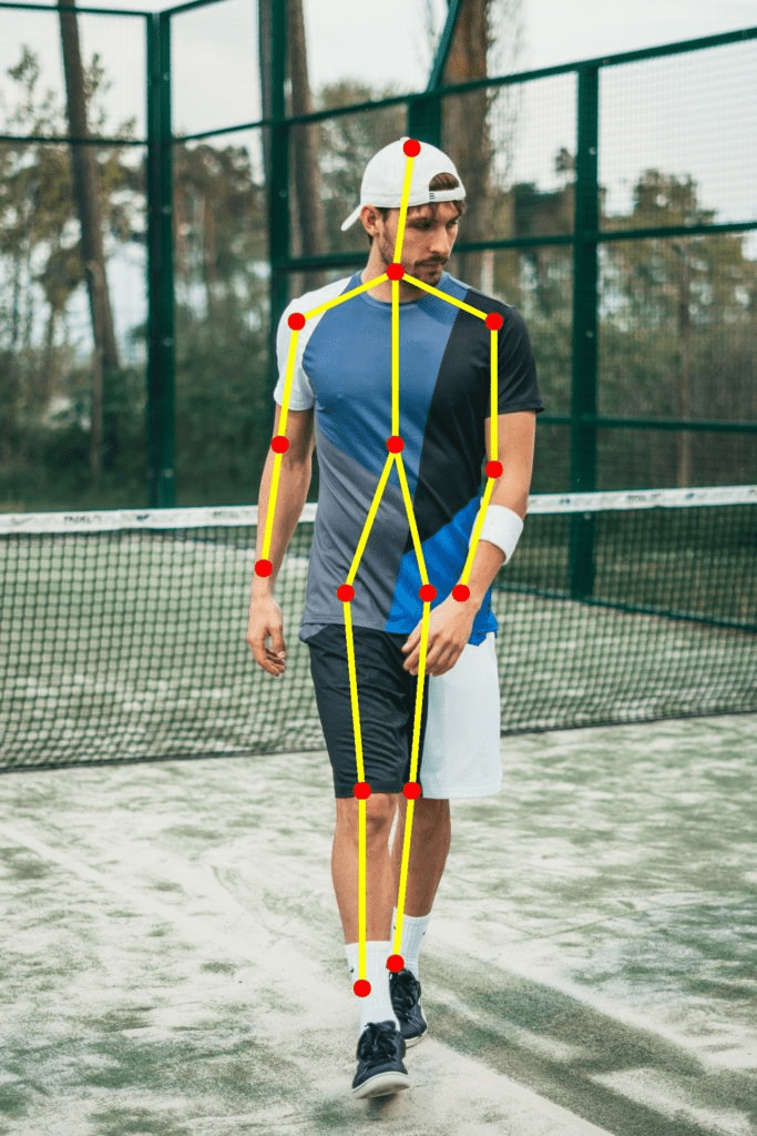
In this article, we will focus on human pose estimation, where it is required to detect and localize the major parts/joints of the body ( e.g. shoulders, ankle, knee, wrist etc. ). Remember the scene where Tony stark wears the Iron Man suit using gestures? If such a suit is ever built, it would require human pose estimation! For the purpose of this article, though, we will tone down our ambition a tiny bit and solve a simpler problem of detecting keypoints on the body. A typical output of a pose detector looks as shown below :
Keypoint detection datasets
Until recently, advancement in pose estimation has been challenged because of the lack of high-quality datasets. Such is the enthusiasm in AI these days that problems that would not have been addressed are now within reach. Exciting new datasets have been released in the last few years which have made it easier for researchers to attack wider opportunities with all their intellectual might.
Some of the datasets are :
- COCO Keypoints challenge
- MPII Human Pose Dataset
- VGG Pose Dataset
In short the more images a system sees the better and more intelligent it gets.
2. Multi-person pose estimation model
The model used in this tutorial is based on a paper titled Multi-Person Pose Estimation by the Perceptual Computing Lab at Carnegie Mellon University. The authors of the paper train very deep neural networks for this task. Let’s briefly go over the architecture before we explain how to use the pre-trained model.
The model takes as input a color image of size w × h and produces, as output, the 2D locations of keypoints for each person in the image. The detection takes place in three stages :
Stage 1: The first 10 layers of the VGGNet are used to create feature maps for the input image.
Stage 2: A 2-branch multi-stage CNN is used where the first branch predicts a set of 2D confidence maps (S) of body part locations ( e.g. elbow, knee etc.). Given below are confidence maps and Affinity maps for the keypoint Left Shoulder.

The second branch predicts a set of 2D vector fields (L) of part affinities, which encode the degree of association between parts. In the figure below part affinity between the Neck and Left shoulder is shown.

Pre-trained models for human pose estimation
The authors of the paper have shared two models – one is trained on the Multi-Person Dataset ( MPII ) and the other is trained on the COCO dataset. The COCO model produces 18 points, while the MPII model outputs 15 points. The outputs plotted on a person is shown in the image below.
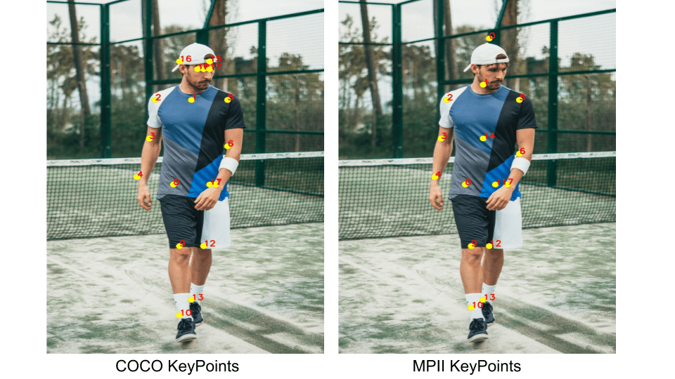
COCO output format Nose – 0, Neck – 1, Right Shoulder – 2, Right Elbow – 3, Right Wrist – 4, Left Shoulder – 5, Left Elbow – 6, Left Wrist – 7, Right Hip – 8, Right Knee – 9, Right Ankle – 10, Left Hip – 11, Left Knee – 12, Left Ankle – 13, Right Eye – 14, Left Eye – 15, Right Ear – 16, Left Ear – 17, Background – 18 MPII Output Format Head – 0, Neck – 1, Right Shoulder – 2, Right Elbow – 3, Right Wrist – 4, Left Shoulder – 5, Left Elbow – 6, Left Wrist – 7, Right Hip – 8, Right Knee – 9, Right Ankle – 10, Left Hip – 11, Left Knee – 12, Left Ankle – 13, Chest – 14, Background – 15
As we saw in the previous section that the output consists of confidence maps and affinity maps. These outputs can be used to find the pose for every person in a frame if multiple people are present.
The output is a 4D matrix :
- The first dimension being the image ID ( in case you pass more than one image to the network ).
- The second dimension indicates the index of a keypoint. The model produces Confidence Maps and Part Affinity maps which are all concatenated. For COCO model it consists of 57 parts – 18 keypoint confidence Maps + 1 background + 19*2 Part Affinity Maps. Similarly, for MPI, it produces 44 points. We will be using only the first few points which correspond to Keypoints.
- The third dimension is the height of the output map.
- The fourth dimension is the width of the output map.
We check whether each keypoint is present in the image or not. We get the location of the keypoint by finding the maxima of the confidence map of that keypoint. We also use a threshold to reduce false detections.
Once the keypoints are detected, we just plot them on the image. Since we know the indices of the points before-hand, we can draw the skeleton when we have the keypoints by just joining the pairs.
This is how we are able to detect what is taking place in the video whether it is an individual or multiple person feed.